
Speaker Diarization enables speakers in an adverse acoustic environment to be accurately identified, classified, and tracked in a robust manner. There are many intricacies involved in developing a speaker diarization system. VOCAL’s speaker diarization software, when combined with our beamforming module, provides automatic detection, classification, isolation, and tracking of a given speaker source. Please contact us for details concerning your specific speech application.
Source Diarization
Source Diarization is the process of determining how many distinct signal sources are present within a given data stream. For speech applications, we can utilize these techniques to determine how many speakers are present in a given audio segment.
Speech Detection is typically done using a learning model. A popular choice in the past has been Gaussian Mixture Models, or Hidden Markov Models. Typically, distortions such as noise or music are explicitly modeled as distinct from speech. To implement such a system, long segments of speech, typically at least one second of data, are required. The audio is segmented with Voice Activity Detection or Viterbi methods, and then the parsed segments are classified as pure speech, some kind of speech mixture or something different.
Once the speech segments have been identified, we need to cluster the data that comes from the same source. Typically, we create a feature vector ![]()
![]() that best explains the speech segment, much like in Voice Activity Detection algorithms, or Speaker Recognition. One of the most popular distance metrics for these vectors used is the Bayesian Information Criteria (BIC):
that best explains the speech segment, much like in Voice Activity Detection algorithms, or Speaker Recognition. One of the most popular distance metrics for these vectors used is the Bayesian Information Criteria (BIC):
![]()
![]() (1)
(1)
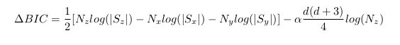
Where M is the model order, N is the number of speech segments being considered, ℒ is the likelihood ratio statistic, and α is a constant. To make the decision, we look at the magnitude of the change in BIC with respect to the current speaker cluster x, the other speaker cluster y and the parent cluster z, which represents the decision that speakers x and y are actually the same speaker z. It is computed via:
 (2)
(2)
Where d is the dimension of the feature vector ![]()
![]() being considered. Once all the speakers are clustered, a second pass can be taken to reduce the number of clusters, in other words, to make sure the decisions represent reality. To do so, we compute the cross-likelihood ration (CLR) via:
being considered. Once all the speakers are clustered, a second pass can be taken to reduce the number of clusters, in other words, to make sure the decisions represent reality. To do so, we compute the cross-likelihood ration (CLR) via:
![]()
![]() (3)
(3)
Where L(mi |λj) is the average likelihood of data frame mi given cluster λi, and λU is a general speaker cluster created from general speaker training data.
References
[1] S. Tranter, D. Reynolds, “An Overview of Automatic Speaker Diarisation Systems,” IEEE Trans on SAP, 2006