Machine Learning Algorithms are becoming more and more prominent in the audio processing community, as we simultaneously move towards more complicated signal processing models and distributed memory systems. VOCAL’s robust machine learning software provides customers with optimally refined as well as adaptive speech processing discriminants for crisp audio across any environment. A few examples of how VOCAL uses such tools are provided below.
Speech Classification
The task of classifying speech versus interference is a difficult one, yet absolutely integral to the proper functioning of any speech enhancement solution. Parametric approaches to such classification use audio features to segment the signal. Once the features have been identified, we can perform the classification and visualize the ability of the classifier using a confusion matrix, a ROC curve, or a PR curve.
A confusion matrix is a graphical representation of the ability of the classifier to do its job. Basically, it represents how often the classifier makes a mistake. Ideally, a confusion matrix will be diagonal, but practically it will never be entirely so. Instead, we need to make it “as diagonal as possible” such that the diagonal elements are dominant to the other terms. An example of a confusion matrix is shown below:
Prediction outcome
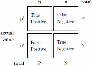
While that is certainly illustrative when the class size is small, or to illustrate the results of an optimization procedure, it is not very helpful in visualizing how well that optimization procedure actually did. Perhaps one type of error dominates over the others on your training set, and perhaps we can choose a different pareto optimal solution that will generalize better. To visualize these tradeoffs, we create what is called a Receiver Operator Characteristics Curve shown below:
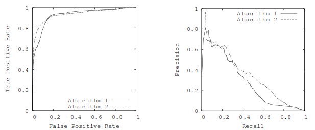
Figure 1: ROC and PR Curves [1]
ROC Curves measure the tradeoff between true and false positives. Ideally, the curve approaches the left most corner, that is, we have high true positive rates with low false positive rates. As you increase the false positive rate, you can see how the true positive rate changes, and vice versa. This can help you find the optimal tradeoff for your given problem. Another way to visualize your classifiers performance is through the Precision/Recall graph shown to the right in the figure above.
Precision is defined as:
![]()
![]() (1)
(1)
While Recall is defined as:
![]()
![]() (2)
(2)
As [1] illustrates, a given classifier will dominate in ROC space iff it is dominant in PR space. Therefore, in some sense, they are equivalent, however, the integral of an ROC curve cannot be given the same interpretation as the integral of the PR curve. Hence, plotting both can give you insight into the classifiers behavior. As [1] shows, sometimes a given algorithm does better than another in ROC space but not PR space.
Applications of Machine Learning
Through over 26 years of experience, VOCAL can leverage information about countless scenarios, for instance, to create a robust speech classifier. Other machine learning methods have been applied to optimize and adapt filter coefficients in other algorithms such as echo cancellation and dereverberation. In addition, beamforming can be done parametrically to harness the depth and breadth of VOCAL’s knowledge of audio. VOCAL has successfully applied machine learning techniques to improve upon state of the art methodologies for solving your speech quality problems.
References
[1] J. Davis, M. Goadrich. The relationship between precision-recall and roc curves. Technical report # 1551, University of Wisconsin Madison, January 2006