Polynomial Interpolation | VOCAL Technologies

Polynomial interpolation is a classical approach to estimating a signal which passes through a set of known points. Consider an example where there is a data set consisting of N+1 samples $\left [ x(t_{0}), x(t_{1}), \cdots, x(t_{N})\right ]$ . Polynomial interpolators can be formulated as a power series using a set of calculated polynomial coefficients $\left [ a_{0}, a_{1}, \cdots , a_{N}\right ]$ . The equation of the interpolated signal which passes through points $\left [ x(t_{0}), x(t_{1}), \cdots , x(t_{N})\right ]$ is given as:

$\hat{x}(t) = a_{0} + a_{1}t + a_{2}t^{2}+a_{3}t^{3}+\cdots +a_{N}t^{N}$ (1.1)

From the previous equation, x at time $t_k$ can be calculated as:

$x(t_{k}) = a_{0} + a_{1}t + a_{2}t_{k}^{2}+a_{3}t_{k}^{3}+\cdots +a_{N}t_{k}^{N}$ (1.2)

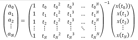
Therefore, the polynomial coefficients are given by:

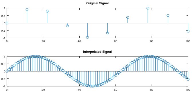
The signal can be interpolated using the obtained coefficients in equation 1.1. This concept is demonstrated in the below figure. The original signal contains 11 samples. The signal obtained from interpolation is much higher resolution (101 samples), and is able to accurately represent the original waveform. This method can be suitable for interpolation of a small number of samples. For a larger number of samples N+1, quantization errors can cause the interpolation of the signal to be inaccurate.

Complete Communications Engineering