Bayesian Filtering | VOCAL Technologies

Bayesian filtering is a method for solving optimal filtering problems using Bayesian probability theory to estimate the state of a time-varying process or system which is observed through a noise-polluted signal. The state of a system refers to a collection of parameters which describe the behavior of a system. In Bayesian filtering problems, the state of the system is typically modeled as a Markovian chain with associated transition probabilities between states (see Appendix A).

Bayesian filtering is essentially a statistical inversion problem where a desired vector x must be estimated based on an observed signal y which is the summation of vector x with added noise. The goal is to use the observed sequence to produce an estimation of the hidden states. To do this in the Bayesian sense, this simply implies that the joint posterior PDF of all states given all observations must be computed,

$p(\textbf{x}_{k}|\textbf{y}_{1:k}) = \frac{p(y_{k}|x_{k})p(x_{k}|y_{1:k-1})}{Z_{k}}$ (eq. 1.1)

$p(x_{k}|y_{1:k-1})$ is the predictive distribution of the state of $\mathbf{x}$ at time interval k, which can be calculated using the Chapman-Kolmogorov in eq. 1.2. $p(\mathbf{y}_{k}|\mathbf{x}_{k})$ is the likelihood model for the observed sequence given $\mathbf{x}$ , and $Z_{k}$ is the normalization factor. Using eq. 1.1, Bayesian filtering problems compute the marginal posterior PDF of state $\mathbf{x}$ at each time interval k given the previous history of observations up to time k. Application which apply Bayesian theory, such as Kalman filters, can be implemented using the following procedure:

1. Initialization: Assume an initial state from the given prior distribution $p(\mathbf{x}_{0})$

2. Prediction: The predictive distribution of the state of x is calculated as follows.

$p(\mathbf{x}_{k}|\mathbf{y}_{1:k-1}) = \int p(\mathbf{x}_{k}|\mathbf{x}_{k-1})p(\mathbf{x}_{k-1}|\mathbf{y}_{1:k-1})d\mathbf{x}_{k}$ (eq. 1.2)

3. Update: From measurement $\mathbf{y}_{k}$ at time interval k, the posterior PDF is calculated using eq 1.1, where the normalization constant can be calculated as:

$Z_{k} = \int p(\mathbf{y}_k|\mathbf{x}_k)p(\mathbf{x}_{k}|\mathbf{y}_{1:k-1})d\mathbf{x}_{k}$ (eq. 1.3)

Appendix A: Markovian Chains

Hidden Markov models (HMMs) are statistical-based models which can be used to prototype the behavior of non-stationary signal processes such as time-varying image sequences, music signals, and speech signals. Non-stationary characteristics of speech signals include two main categories: variations in spectral composition and variations in articulation rate. An HMM considers the probabilities associated with state observations and state transitions to model these variations.

Consider the speech signal as shown in Figure 1 below. The respective segments of the given signal can be modeled by a Markovian state. Each state must consider the random variations that can occur in the different realizations of the signal by having probabilistic events which represent the state observation probabilities. The transition probabilities between each state provide a connection between the HMM states. When a given probabilistic event occurs, the state will transition to the next state in the HMM. Conversely, the state may self-loop rather than transition if a different probabilistic event occurs which does not imply transition.

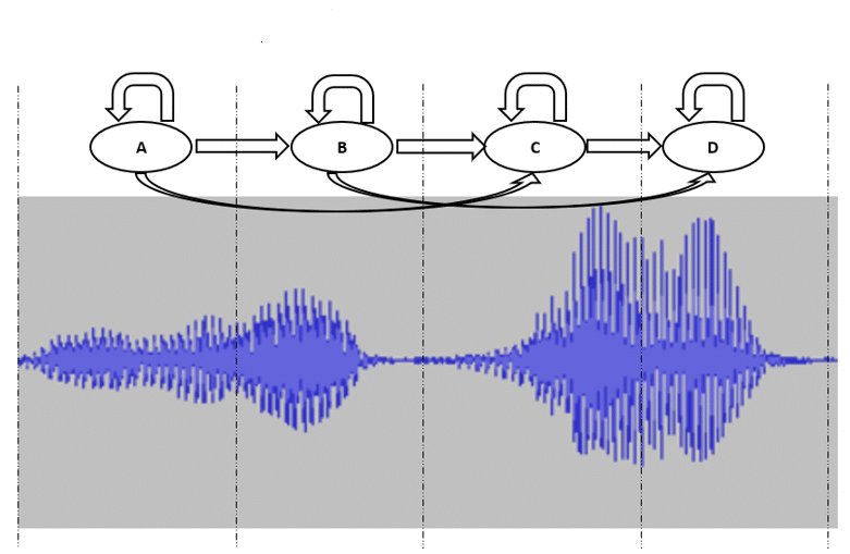
Figure 1: HMM speech model example

Complete Communications Engineering

Appendix A: Markovian Chains