Basics of Kalman Filters

The Kalman filter is a Bayesian-based recursive least square error method which can be used to estimate a signal or parameter which is riddled with noise. Essentially, given some noisy observation signal, the Kalman filter is able to de-noise a signal by iterating through two recursive stages: the update stage, and the estimation stage. In the update stage, the state of the signal is predicted from previously made observations and a prediction error covariance matrix is computed. In the estimation stage, using the previously made observations, the Kalman gain coefficient is calculated. The estimation error covariance matrix to be used in the next iteration is then computed using the obtained Kalman gain coefficient. This process repeats until the Kalman gain coefficient is tuned to the proper value for the system. The result is an estimation of the desired signal with minimal noise.

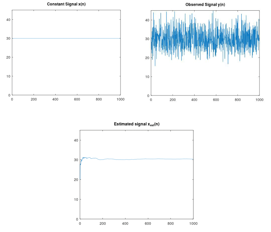
Kalman filters can be applied to both time invariant and time-varying signals. For simplicity, consider a simple example where there is a constant signal contaminated with noise and must be estimated. The initial conditions are established below in (1) and (2). For this example, the current state of the signal is unknown, therefore the variance will be assumed to be a very large value. Given the observations, the next value of the signal is predicted in the update stage, then an estimation of the signal is made after the computation of the Kalman gain coefficient.

(1) $x(m) = x(m-1) = x$ (constant signal)
(2) $y(m) = x + n(m)$ (observed signal with white noise)

Initial Conditions:
Previous estimated value: $\hat{x}(0|-1) = 0$
Previous Cov() of prediction error: $P (-1) = 1000$

Update stage:
Signal prediction: $\hat{x}(m|m-1) = \hat{x}(m-1)$
Cov() of prediction error: $P(m|m-1) = P(m-1)$

Estimation stage:
Kalman gain computation: $K(m) = P(m|m-1)(P(m|m-1)+\sigma _{n}^{2})^{-1}$
Estimation of signal: $\hat{x}(m) = \hat{x}(m|m-1)+K(m)(y(m)-\hat{x}(m|m-1))$
Covariance re-calculation: $P(m) = (1-K(m))P(m|m-1)$

The results of the Kalman filter algorithm are shown in the below figures. As the algorithm iterates, the Kalman gain is adjusted based on the information from the observed signal and an accurate estimation of the original signal is obtained in the final figure. This application can be adjusted for autoregressive processes, and applied to non-stationary signals such as speech.

Complete Communications Engineering