For a general microphone array, each element has a response to a source that is a function of the source direction. For the direction  , we denote the response as
 ") from the microphone m. If K sources exist, we have the spatial matrix below,
from the microphone m. If K sources exist, we have the spatial matrix below,
![A\ =\left[\begin{matrix}a_1\left(\theta_1\right)&\cdots&a_1\left(\theta_K\right)\\\vdots&\ddots&\vdots\\a_M\left(\theta_1\right)&\cdots&a_M\left(\theta_K\right)\\\end{matrix}\right]](https://s0.wp.com/latex.php?latex=A%5C+%3D%5Cleft%5B%5Cbegin%7Bmatrix%7Da_1%5Cleft%28%5Ctheta_1%5Cright%29%26%5Ccdots%26a_1%5Cleft%28%5Ctheta_K%5Cright%29%5C%5C%5Cvdots%26%5Cddots%26%5Cvdots%5C%5Ca_M%5Cleft%28%5Ctheta_1%5Cright%29%26%5Ccdots%26a_M%5Cleft%28%5Ctheta_K%5Cright%29%5C%5C%5Cend%7Bmatrix%7D%5Cright%5D&bg=ffffff&fg=000000&s=0 "A\ =\left[\begin{matrix}a_1\left(\theta_1\right)&\cdots&a_1\left(\theta_K\right)\\\vdots&\ddots&\vdots\\a_M\left(\theta_1\right)&\cdots&a_M\left(\theta_K\right)\\\end{matrix}\right]")
and the microphone array output,
![\left[\begin{matrix}x_1\left(t\right)\\\vdots\\x_M\left(t\right)\\\end{matrix}\right]=\left[\begin{matrix}a_1\left(\theta_1\right)&\cdots&a_1\left(\theta_K\right)\\\vdots&\ddots&\vdots\\a_M\left(\theta_1\right)&\cdots&a_M\left(\theta_K\right)\\\end{matrix}\right]\left[\begin{matrix}s_1\left(t\right)\\\vdots\\s_K\left(t\right)\\\end{matrix}\right]+\left[\begin{matrix}n_1\left(t\right)\\\vdots\\n_M\left(t\right)\\\end{matrix}\right]](https://s0.wp.com/latex.php?latex=%5Cleft%5B%5Cbegin%7Bmatrix%7Dx_1%5Cleft%28t%5Cright%29%5C%5C%5Cvdots%5C%5Cx_M%5Cleft%28t%5Cright%29%5C%5C%5Cend%7Bmatrix%7D%5Cright%5D%3D%5Cleft%5B%5Cbegin%7Bmatrix%7Da_1%5Cleft%28%5Ctheta_1%5Cright%29%26%5Ccdots%26a_1%5Cleft%28%5Ctheta_K%5Cright%29%5C%5C%5Cvdots%26%5Cddots%26%5Cvdots%5C%5Ca_M%5Cleft%28%5Ctheta_1%5Cright%29%26%5Ccdots%26a_M%5Cleft%28%5Ctheta_K%5Cright%29%5C%5C%5Cend%7Bmatrix%7D%5Cright%5D%5Cleft%5B%5Cbegin%7Bmatrix%7Ds_1%5Cleft%28t%5Cright%29%5C%5C%5Cvdots%5C%5Cs_K%5Cleft%28t%5Cright%29%5C%5C%5Cend%7Bmatrix%7D%5Cright%5D%2B%5Cleft%5B%5Cbegin%7Bmatrix%7Dn_1%5Cleft%28t%5Cright%29%5C%5C%5Cvdots%5C%5Cn_M%5Cleft%28t%5Cright%29%5C%5C%5Cend%7Bmatrix%7D%5Cright%5D&bg=ffffff&fg=000000&s=0 "\left[\begin{matrix}x_1\left(t\right)\\\vdots\\x_M\left(t\right)\\\end{matrix}\right]=\left[\begin{matrix}a_1\left(\theta_1\right)&\cdots&a_1\left(\theta_K\right)\\\vdots&\ddots&\vdots\\a_M\left(\theta_1\right)&\cdots&a_M\left(\theta_K\right)\\\end{matrix}\right]\left[\begin{matrix}s_1\left(t\right)\\\vdots\\s_K\left(t\right)\\\end{matrix}\right]+\left[\begin{matrix}n_1\left(t\right)\\\vdots\\n_M\left(t\right)\\\end{matrix}\right]")
or
=A\left(\theta\right)s\left(t\right)+n\left(t\right)")
the snapshot of the array at time t.
The snapshot contains certain structures of the data model. Pack a block of snapshots of length L into a matrix,
![X(t)=\left[\left[\begin{matrix}x_1\left(t\right)\\\vdots\\x_M\left(t\right)\\\end{matrix}\right]\ldots\ \left[\begin{matrix}x_1\left(t+L\ -\ 1\right)\\\vdots\\x_M\left(t+L\ -\ 1\right)\\\end{matrix}\right]\right]](https://s0.wp.com/latex.php?latex=X%28t%29%3D%5Cleft%5B%5Cleft%5B%5Cbegin%7Bmatrix%7Dx_1%5Cleft%28t%5Cright%29%5C%5C%5Cvdots%5C%5Cx_M%5Cleft%28t%5Cright%29%5C%5C%5Cend%7Bmatrix%7D%5Cright%5D%5Cldots%5C+%5Cleft%5B%5Cbegin%7Bmatrix%7Dx_1%5Cleft%28t%2BL%5C+-%5C+1%5Cright%29%5C%5C%5Cvdots%5C%5Cx_M%5Cleft%28t%2BL%5C+-%5C+1%5Cright%29%5C%5C%5Cend%7Bmatrix%7D%5Cright%5D%5Cright%5D&bg=ffffff&fg=000000&s=0 "X(t)=\left[\left[\begin{matrix}x_1\left(t\right)\\\vdots\\x_M\left(t\right)\\\end{matrix}\right]\ldots\ \left[\begin{matrix}x_1\left(t+L\ -\ 1\right)\\\vdots\\x_M\left(t+L\ -\ 1\right)\\\end{matrix}\right]\right]")
and the data
The covariance matrix, ![R_y=E\left[YY^H\right]=AR_sA^H+R_n](https://s0.wp.com/latex.php?latex=R_y%3DE%5Cleft%5BYY%5EH%5Cright%5D%3DAR_sA%5EH%2BR_n&bg=ffffff&fg=000000&s=0 "R_y=E\left[YY^H\right]=AR_sA^H+R_n") , is Hermitian and positive definite since
, is Hermitian and positive definite since  is always positive definite.
This short paper the basic idea and implementation are described. Its use for resolving multiple sound sources with antenna array is discussed.
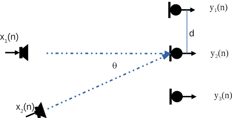
Generalizing Figure 1 to N sources to M microphones, we have the microphone captured sound vector,
=\sum_{n=1}^{N}{s_n\ \left(t\right)e^{-j2\pi f\left(m-1\right)dsin\left(\theta_n\right)/v}}+noise_m\left(t\right) =\sum_{n=1}^{N}")
a_m\left(\theta_n\right)}+noise_m\left(t\right)")
We can further write this into the following matrix form,

where ![Y = \left[y 1\left(t\right), y 2\left(t\right), \dots , y M\left(t\right)\right], S = \left[s1\left(t\right), s 2 \left(t\right), \dots , s N \left(t\right)\right]](https://s0.wp.com/latex.php?latex=Y+%3D+%5Cleft%5By+1%5Cleft%28t%5Cright%29%2C+y+2%5Cleft%28t%5Cright%29%2C+%5Cdots+%2C+y+M%5Cleft%28t%5Cright%29%5Cright%5D%2C+S+%3D+%5Cleft%5Bs1%5Cleft%28t%5Cright%29%2C+s+2+%5Cleft%28t%5Cright%29%2C+%5Cdots+%2C+s+N+%5Cleft%28t%5Cright%29%5Cright%5D&bg=ffffff&fg=000000&s=0 "Y = \left[y 1\left(t\right), y 2\left(t\right), \dots , y M\left(t\right)\right], S = \left[s1\left(t\right), s 2 \left(t\right), \dots , s N \left(t\right)\right]") , and
, and ![A=\left[a_1\left(\theta_1\right),a_2\left(\theta_2\right),\cdots,a_M\left(\theta_N\right)\right]](https://s0.wp.com/latex.php?latex=A%3D%5Cleft%5Ba_1%5Cleft%28%5Ctheta_1%5Cright%29%2Ca_2%5Cleft%28%5Ctheta_2%5Cright%29%2C%5Ccdots%2Ca_M%5Cleft%28%5Ctheta_N%5Cright%29%5Cright%5D&bg=ffffff&fg=000000&s=0 "A=\left[a_1\left(\theta_1\right),a_2\left(\theta_2\right),\cdots,a_M\left(\theta_N\right)\right]") .
.
The covariance matrix, , is Hermitian and positive definite since is always positive definite.
By eigenvalue decomposition, vi and λi are the eigenvector and corresponding eigenvalue, we have
 .
.
The noise dimension has smaller eigenvalue, which is the noise floor, while the dimensions that contain signals will have larger eigenvalue. Therefore, the noise subspace can be constructed by
![E_N=\left[\mathbf{v}_{\mathbf{N}+\mathbf{1}},\mathbf{v}_{\mathbf{N}+\mathbf{2}},\cdots,\mathbf{v}_\mathbf{M}\right]](https://s0.wp.com/latex.php?latex=E_N%3D%5Cleft%5B%5Cmathbf%7Bv%7D_%7B%5Cmathbf%7BN%7D%2B%5Cmathbf%7B1%7D%7D%2C%5Cmathbf%7Bv%7D_%7B%5Cmathbf%7BN%7D%2B%5Cmathbf%7B2%7D%7D%2C%5Ccdots%2C%5Cmathbf%7Bv%7D_%5Cmathbf%7BM%7D%5Cright%5D&bg=ffffff&fg=000000&s=0 "E_N=\left[\mathbf{v}_{\mathbf{N}+\mathbf{1}},\mathbf{v}_{\mathbf{N}+\mathbf{2}},\cdots,\mathbf{v}_\mathbf{M}\right]") .
.
The signal dimension will have smaller value if it is projected into the noise subspace. Therefore, the following formula will have larger value and appear to be a peak,
\right|^2}\ =\ \frac{1}{a^H\left(\theta\right)E_nE_n^Ha\left(\theta\right)}")
The above formula defines the MUSIC algorithm. The number of peaks indicates the number of independent sound sources and the corresponding direction \theta defines the incoming direction of each sound source.
It is important to remember that the MUSIC algorithm implementation described there applies to only narrow band signal. The performance of the algorithm also depends on the relation between the inter-mic distance and the sampling frequency.