The wave equation,

is a partial differential equation that describes the disturbance of a medium due to changes in pressure. The solution is often used to describe propagating waves in an acoustic environment. Such a scenario is solved using three main approaches: geometrical acoustics, waved-based techniques, and artificial methods. Here, we will discuss geometric and wave-based methods.
Geometrical acoustics is based on the assumption that sound travels as a particle in a ray instead of a wave. This only holds true when the model dimensions are much greater than the desired wavelengths. The underlying assumption omits any investigated of small room acoustics and low frequencies, leaving only large acoustic spaces. Wave phenomena, such as diffraction, are also unable to be modeled due to the limitations of geometrical acoustics. The most used computational algorithms in geometric techniques are ray-tracing and image-source method.
Wave-based techniques are a more accurate model that can describe wave propagation in a cavity (interior) or from a radiating body (exterior). Unlike geometric techniques, wave phenomena are modeled through numerical techniques including finite-difference time-domain (FDTD), finite element methods (FEM) and boundary element methods (BEM).
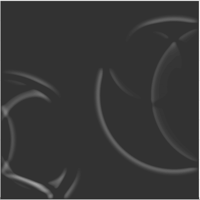
With FDTD, the wave equation is approximated using finite difference equations. The acoustic model is voxelized1 , assigning a finite difference equation to each node of the structure. As seen in Figure 1, the model is iterated through in the time-domain to numerically solve the wave equation. One disadvantage is FDTD’s costly computationally load. Heuristics ask for at least 10 nodes per wavelength, which may require a dense nodal structure for larger models or higher frequency investigation. Nevertheless, new finite difference formulations utilizing parallel programming are constantly being developed to combat this issue.
FEM and BEM use a different methodology, using partial differential equations in order to numerically solve the inhomogeneous wave equation. FEM uses a volumetric structure, discretizing the acoustic model into elements connected by nodes. The unknown functions are solved at each nodal position, allowing for values to be interpolated inside the elements by a geometrically-dependent shape function.
BEM follows the same principle, but only solves for the boundary of the model. This formulation of BEM allows for a natural application in solving radiation and scattering.
In general, FEM requires extensive time building the model; however, the matrices used to solve the partial differential equations are sparse, allowing for more computational efficiency. Conversely, BEM only requires a two-dimensional structure, but the matrices are mathematically dense, making the calculations more intensive. To find a balance between the aforementioned techniques, methods are also being implemented combining geometrical and wave-based techniques.