Nearfield Structure of Acoustic Radiation

Abstract

This white paper categorizes the structure of acoustic radiation fields into three distinct zones: the farfield, the nearfield, and the extreme nearfield (also referred to as the evanescent regime). The farfield is where acoustic waves can be approximated as plane waves. The extreme nearfield is characterized by non-propagating, exponentially decaying fields. In contrast, the nearfield lies between these two extremes and exhibits both spatial complexity and field propagation, making it particularly important for applications involving acoustic trapping and manipulation. Although the applications are briefly addressed, the emphasis of this paper is on explaining the structure of the nearfield zone.

Introduction

Acoustic radiation fields exhibit different structures/behaviors depending on the distance from their source. In this paper, we categorize these behaviors into three distinct zones:

1. Farfield
2. Nearfield
3. Extreme Nearfield (Evanescent Regime)

The emphasis is on the nearfield, though both the farfield and evanescent regime will be introduced to contrast their characteristics with those of the nearfield. Each of these zones can be distinguished by analyzing the spatial components of wave propagation and field complexity.

The Farfield Zone

The farfield of an acoustic wave is defined as the region where the wave can be approximated as a plane wave. A plane wave is a special type of wave in which a physical quantity—such as phase—remains constant across any plane that is perpendicular to the direction of propagation, although this quantity may vary from one such plane to another along the propagation axis. While true plane waves are rarely found in nature, they provide a valuable approximation for describing wave behavior in the farfield. In the context of this white paper, the plane wave propagates in a direction that is almost normal to the surface of an acoustic source. The dominance of propagation along this normal axis, coupled with negligible contributions from lateral components, simplifies the field’s structure.

Many applications occur in the farfield. For example, acoustic sources can be arranged to simulate plane waves approaching from opposite directions. This setup enables the formation of standing waves, which can be exploited for particle levitation. NASA has used this principle to simulate microgravity environments, with levitating particles mimicking microgravity conditions.

Such levitation is essential in studies of drug delivery for astronauts, who experience health risks after prolonged exposure to microgravity. Therefore, research in drug delivery under microgravity conditions is of significant interest.

Mathematical Framework

To provide insight into acoustic wave behavior, we consider a plane wave with a single angular frequency ω₀ propagating at speed c, described by the equation:

Here, p₀ is the acoustic pressure amplitude, and is the wavevector with its magnitude (known as the wavenumber) being defined by:

The Cartesian coordinates x, y and z represent spatial dimensions, while the components and define the wavevector along the respective axes and are thus associated with the wave’s direction of propagation. We assume that the x − y  plane corresponds to the surface of the acoustic source, with the z −axis normal to this surface and representing the direction of propagation.

By keeping the total wavenumber k constant and allowing to k_x and k_y take real values, we can express:

Thus, k_z becomes a function of k_x and k_y The wavevector can also be represented as:  where λ_x, λ_y, and λ_z are the wavelengths along the respective axes.

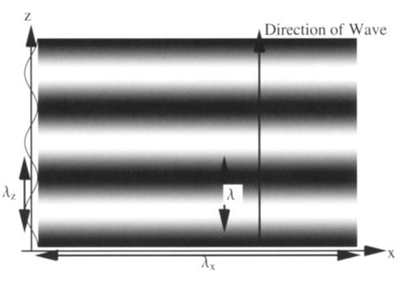
These relations reveal that k_z is dependent on k_x and k_y, which represent transverse wave components. A large axial component (and small transverse ones) implies nearly pure propagation in the z-direction — characteristic of the far field.

In such regions, as k_x → 0 and k_y → 0., the wave propagates primarily in the axial direction, forming plane wavefronts (see Figure 1, where bright and dark bands represent wave crests and troughs respectively).

The Extreme Nearfield (Evanescent Regime)

In the extreme nearfield or evanescent regime, the inequality holds, making k_z a complex number. This results in exponentially decaying radiation, transforming the wave equation to:

Here, the phase term is:

φ = k_xx + k_zz −ω₀t

Exponential decay along the z-axis implies nearly zero propagation, and the evanescent field remains tightly confined to the surface of the source. Although lacking propagation, this regime features highly complex field structures. In fact, several medical applications⁵ have utilized these evanescent fields by placing the target object directly on the source.

The Nearfield Zone

Unlike the farfield or evanescent regimes, the nearfield exhibits both complex structures and propagation. In this region, k_x and k_y are present, but ensuring that k_z remains real and field propagation along the z-axis continues.

As k_z becomes smaller (closer to zero), less propagation and more complexity arise. This complexity is best understood using k-space (the spatial frequency domain), where the acoustic field in the nearfield contains a broad spectrum of spatial frequencies. Each of these frequencies could contribute to a different type of propagation along the axial and lateral axis. This broad spectrum of spatial frequencies result in rapid pressure fluctuations and sharp acoustic gradients,
which are essential for applications requiring strong trapping forces.

To study the field structure, it is insightful to analyze the x-z plane at y=0, where the phase term becomes:

φ = k_xx + k_zz −ω₀t

Plotting this wave at t = 0 yields a result similar to Figure 2.

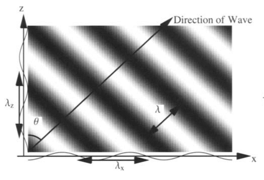
To better understand Figure 2 one may define z as the axis normal to the surface. The wave propagation direction forms an angle θ, such that:

λ_x sin θ = λ

λ_z cos θ = λ

k_x = k sin θ

k_z = k cos θ

This confirms that the wave not only propagates along z but also has wavenumber projections along x.

In this scenario, each k-space can be associated to a plane wave, which can be analyzed using numerical models such as the Angular Spectrum Method (ASM). ASM helps determine how each wave contributes to the total field structure. By decomposing the field this way, one can understand and exploit high spatial frequencies for applications requiring sharp gradients and high localization.

Although Figure 2 is two-dimensional, similar projections exist along the y-axis. Due to the source’s proximity and the wide frequency content, such projections dominate in the nearfield and introduce complex spatial patterns. This complexity creates opportunities for particle manipulation and lens design utilizing nearfield behavior.

Applications and Trends

Acoustic trapping refers to the use of spatially structured sound fields to confine and manipulate particles within a region of acoustic force. Devices that accomplish this are known as acoustic tweezers, and they can be used in biomedical applications, such as guiding chemotherapy agents to targeted tissue sites.

Historically, most acoustic tweezers have operated in the farfield. For instance, Chen et al³. demonstrated the manipulation of various particles using a Single Beam Acoustic Tweezer (SBAT). By adjusting the center frequency and beamwidth of an Ultra High Frequency (UHF) transducer in the farfield, they achieved precise particle control for biomedical use.

Other studies have explored the use of evanescent fields. Although these fields exhibit rich structural detail, they do not support true wave propagation, limiting their practical effectiveness. As a result, attention has increasingly shifted to the nearfield, which uniquely combines high structural complexity with real wave propagation.

Notably, Lirette et al^4,6 utilized nearfield acoustic tweezers to manipulate and extract droplets at liquid-liquid interfaces. In 2022, they extended this work to demonstrate the control of hydrocarbon droplets using nearfield traps that formed dual confinement zones.

These developments underscore the potential of nearfield acoustic fields to achieve fine-tuned manipulation of particles with diverse sizes and properties, offering promising capabilities for biomedical research and precision therapeutics.

Conclusion

This white paper has detailed a classification of acoustic radiation field zones—farfield, nearfield, and extreme nearfield—highlighting their unique structures and potential applications. The nearfield stands out for its balance of propagation and complexity, making it an ideal candidate for next-generation applications in trapping, manipulation.

References

1. Sina Rostami, The characterization of radiation forces using tunable acoustic lenses, (Oxford, University of Mississippi , 2025).

2. Y. Lee, and E. G. Williams, “Nearfield acoustic holography: I. Theory of generalized holography and the development of NAH,” Journal of the Acoustical Society of America 78, 1395–1413 (1985). doi:10.1121/1.392911

3. R. Lirette, and J. Mobley, “Ultrasonic near-field based acoustic tweezers for the extraction and manipulation of hydrocarbon droplets,” , doi: 10.1063/5.0122269. doi:10.1063/5.0122269

4. P. Y. Gires, and C. Poulain, “Near-field acoustic manipulation in a confined evanescent Bessel beam,” , doi: 10.1038/s42005-019-0191-z. doi:10.1038/s42005-019-0191-z

5. R. Lirette, J. Mobley, and L. Zhang, “Ultrasonic Extraction and Manipulation of Droplets from a LiquidLiquid Interface with Near-Field Acoustic Tweezers,” Phys Rev Appl 12, 061001 (2019). doi:10.1103/PhysRevApplied.12.061001

6. X. Chen, K. Ho Lam, R. Chen, Z. Chen, P. Yu, Z. Chen, K. Kirk Shung, et al., “An Adjustable Multi-Scale Single Beam Acoustic Tweezers Based on Ultrahigh Frequency Ultrasonic Transducer,” Biotechnol. Bioeng 114, 2637–2647 (2017). doi:10.1002/bit.26365/abstract