FIR filter design is an indispensible tool in any engineer’s toolkit. In general, there are two main classifications of FIR filter design techniques, namely, suboptimal and optimal methods. The suboptimal technique most often employed is the Window Method, while the two most employed optimal techniques center around the error function we choose to minimize. Here, we will examine all three techniques in detail.
FIR Filter
In general, a causal FIR filter takes the form:
H(ejωT) = b0 + b1 · e-jωT + … + bM-jMωT
(1)
Where h[n] = bn, and bi = ±bM-i for the symmetric and anti-symmetric case respectively.
Here, we would like an algorithm to specify a filter response HI(ejωT) and return a set of coefficients b→ whose magnitude spectrum matches HI exactly. For clarity, we are looking to complete the tuple (HI ; b→).
To design an ideal filter, we need to specify δ1, δ2, ωp and ωs, which represent the passband ripple, the stopband attenuation, the passband cutoff, the and stopband starting frequency respectively. A typical example is δ1 = 0:01dB, δ2 = 90dB, ωp = π/4 , and ωs = π/2. Once this is decided upon, we can move into the specifics of the filter design methods.
The Window Method
All FIR filter design algorithms attempt to represent ideal brick wall filters as compactly as possible in the time domain. Brick wall filters in the frequency domain result in infinitely long syncs in the time domain. For practical implementation, this is a non-starter, so we need to instead approximate the brick wall via a finite number of coefficients in the time domain. The ways to do this are many, however, we must first understand what it means to design an ideal filter. Consider the image below:

Figure 1: Ideal filter specifications for a brick wall filter
The Window Method is one of the quickest design methods around, and offers the most options for designing your filters. Once the parameters are selected as above, we need to create our ideal filter. To create the ideal lowpass:
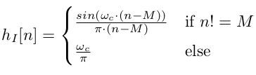
(2)
From here, we multiply our ideal filter with a window function. This results in convolution in the frequency domain, essentially widening the transition width of our ideal filter, and decreasing our stop band attenuation. One widely used family of windows are the Kaiser windows, which are a one parameter family of windows, whose instances approximate the optimal Discrete Prolate Spheroidal Sequence:
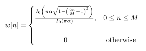
(3)
In other words, the resulting filter h[n] is given by:
h[n] = (w · hI)[n]
(4)
Optimal FIR Filter Design
Optimal filter design chooses to minimize some error representation. The two most common error functions are the least squares, aka L2 norm, and the minimax criterion, aka the infinity norm. Recall that the frequency response of our previously specified ideal filter is given by HI, and suppose our current filter is described by the tuple (HI ; b→). Then, we can create the error function:
![]()
![]()
(5)
We then discretize the problem and create our two optimizations:
![]()
![]() (6)
(6)
![]()
![]() (7)
(7)
Where Ω represents the set of frequencies whose magnitudes are specified by the ideal filter.
The first problem can be solved by standard least squares methods, and the second is usually done via employing the Remez Exchange Algorithm as first done by Parks and McClellan. The advantage of the first optimization is a lower mean squared error, while the advantage of the second is that it will result in a equiripple filter. The decision of which design criteria is best is up to the system specifications, but in general, these optimizations can produce much higher quality filters for the same number of taps compared to suboptimal methods like the Window Method.
FIR Filter Design Considerations
Although the Window Method is a fast, cheap, and popular filter design method for any kind of filter, the method gives a poor result for a low order because the frequency resolution (the main lobe width) of the window function is poor when it is specified with a low number of taps. Therefore, this method will shine for long filter lengths. In contrast, an optimal design targeting the lowest mean squared error or lowest maximum deviation from specification can produce incredibly high quality filters for a low number of taps. The issue with these design methods is that the resulting optimization problems are not trivial to solve, and therefore require either specialized optimization routines, or at the very least, a robust linear equation solver.