In DSP applications when performing audio stream acquisition (and specifically when more than one stream is collected simultaneously) using two (or more) data collection devices that are not driven by the same master clock, streams may be misaligned due to the clock rate differences (however small they might be). Also, when the streams are very long there are chances that some signal samples are missing or redundant samples are inserted into streams at random times, which may happen due to limitations of the data acquisition hardware and/or software.

In audio lab practice when working with multi-microphone systems (for example when collecting audio data from a smart-phone like prototype or development systems), any microphone stream misaligned during the audio data acquisition process, may have a devastating impact on the numerical simulation of audio algorithms that use this experimental data. As such, it is important to verify whether two files are correctly aligned.
There are several techniques for verifying the audio file alignment. Irrespective of the details, any of these techniques can be treated as a specific case of dynamic time warping. Before we go to examples of specific techniques used for file alignment verification and correction, we start with outlining an audio data acquisition system that leads to audio data misalignment.
Sliding Window Method
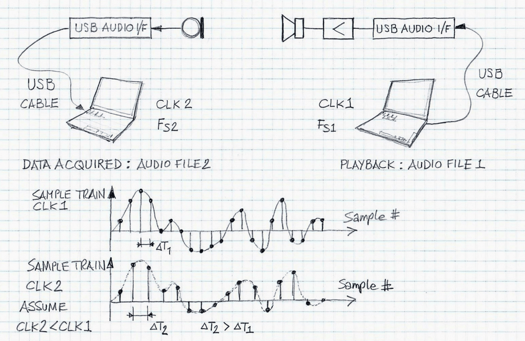
Figure 1 depicts one of the examples, the sliding window method, of such a system. In Figure 1 (and elsewhere) it is assumed that the clock rate, CLK1, is greater than CLK2. Hence, the sampling interval DT2 is greater than DT1.

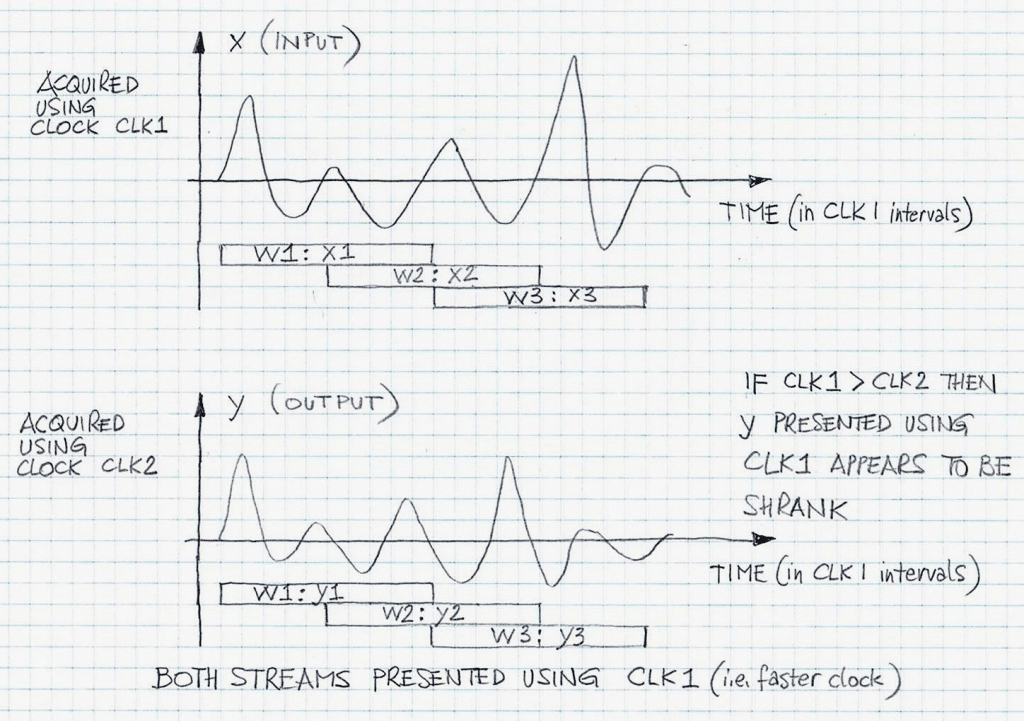
Figure 2 illustrates a sliding window approach for computing the time relationship between audio data segments {x1,y1}, {x2,y2}, …, {xk,yk} in sliding widows w1, w2,…,wk, respectively. The window overlap is 50%. Both waveform plots are drawn using CLK1 rate. Thus, waveform y (output) is shrunk when compared to waveform x (input).
Cross-Correlation Method
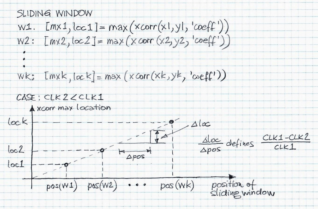
Figure 3 illustrates an approach to determine similarity between audio data segments {x1,y1}, {x2,y2}, …, {xk,yk} based on the cross-correlation function. The graph linking the location of the individual cross-correlation data based on {xj,yj}, j=1,2,…,k. is drawn under the assumption that the clock rate, CLK1, is greater than CLK2. Otherwise, instead of having ascending data points, {pos(wj),xloc} , j=1,2,…,k, we will have ascending data points.

Similar data processing results can be obtained when using an adaptive filter approach, for example using the NLMS algorithm. Then the only additional consideration that has to be taken into account, namely, that the data for the “echo” has to be delayed with respect to the data for the “reference”. Otherwise, the remaining computational details are fairly similar. Specifically, instead of max(xcorr(.)), max(echo_replica(.)) needs to be computed for the individual windows {wj}, j=1,2,…,k. The notation used in Figure 3 include [., .] = max(xcorr(.,., ‘coeff’)), where [., .] represents the max value and location of the max value of the normalized cross-correlation function xcorr(.,., ‘coeff’) (with ‘coeff’ tag indicating the normalization to 1), respectively.
The slope of the ascending data points, {pos(wj),xloc} , j=1,2,…,k, in an ideal case (meaning, no data is corrupted, with the exception of time scale change due to clock rate differences) determines the relative clock rate difference, RCRD, expressed as:
Once that quantity is determined by interpolating {pos(wj),xloc} , j=1,2,…,k, using a linear best-fit function, audio data {y} can be brought to the {x} time scale (determined by CLK1 that is used as a reference of choice) by using the re-sampling technique, as typically employed in DSP-based data processing.
VOCAL’s Voice Enhancement solutions’ engineering practices include analyses and verification of laboratory audio data using various DSP-based techniques such the ones described in this note. Contact us to discuss your audio application.