Hidden Markov Models | VOCAL Technologies

Hidden Markov models (HMMs) are statistical-based models which can be used to prototype the behavior of non-stationary signal processes such as time-varying image sequences, music signals, and speech signals. Non-stationary characteristics of speech signals include two main categories: variations in spectral composition and variations in articulation rate. An HMM considers the probabilities associated with state observations and state transitions to model these variations.

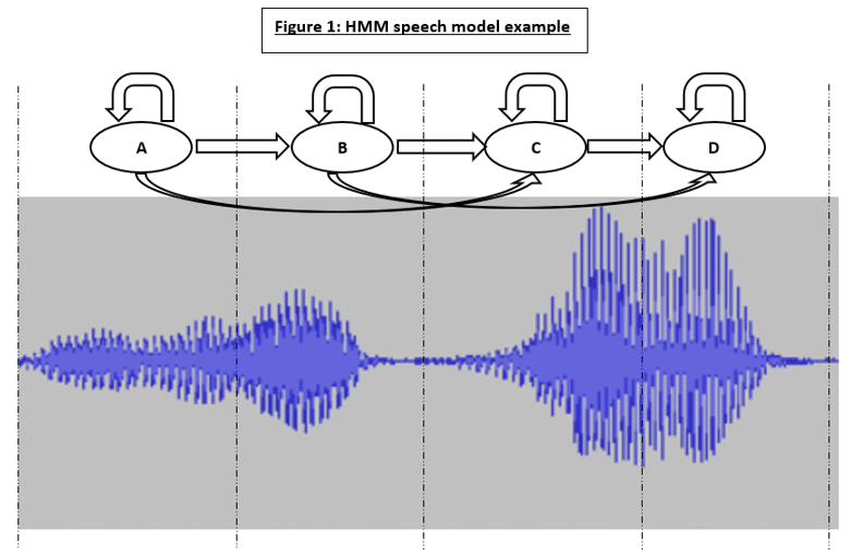
Consider the speech signal as shown in Figure 1 on the following page. The respective segments of the given signal can be modeled by a Markovian state. Each state must consider the random variations that can occur in the different realizations of the signal by having probabilistic events which represent the state observation probabilities. The transition probabilities between each state provide a connection between the HMM states. When a given probabilistic event occurs, the state will transition to the next state in the HMM. Conversely, the state may self-loop rather than transition if a different probabilistic event occurs which does not imply transition.

As an example, consider the use of HMMs in the estimation of a signal x(t) from an observed signal y(t) which is contaminated with noise n(t):

$\mathbf{y}(t) = \mathbf{x}(t) + \mathbf{n}(t)$ (eq. 1.1)

From Bayesian theory, the posterior PDF of the signal x(t) is proportional to the product of the likelihood of observation y(t) given x(t), and the prior PDF function $f_X$ at value x(t):

$f_{X|Y}(\mathbf{x}(t)|\mathbf{y}(t)) = \frac{f_{X|Y}(\boldsymbol{y}(t)|\mathbf{x}(t))f_{X}(\mathbf{x}(t)) }{f_{Y}(\mathbf{y}(t))} = \frac{f_{N}(\mathbf{y}(t)-\mathbf{x}(t))\mathbf{x}(t))f_{X}(\mathbf{x}(t))}{f_{Y}(\mathbf{y}(t))}$

Recall that the maximum a posteriori (MAP) estimate corresponds to the value in which the posterior function obtains a maximum value. The MAP is the value which minimizes the Bayesian risk function, which is defined as the cost error function averaged over all values of the $\mathbf{x}(t)$ . Using the given information and the previous principles of Bayesian theory, the maximum a posteriori estimate (MAP) can be obtained using the following equation:

$\hat{x}^{MAP}(t) = arg_{x(t)}maxf_{N}(\mathbf{y}(t)-\mathbf{x}(t))f_x(x(t))$ (eq. 1.3)

To compute the MAP estimate in eq. 1.3, the PDF models for the signal $\mathbf{x}(t)$ and the noise signal $\mathbf{n}(t)$ are needed. For applications involving time-varying signals such as speech, an N state HMM can be used to model the PDF of the non-stationary process via a Markovian chain of N stationary sub-processes, where each state is trained to model a unique section of a given process. For the problem of signal estimation, it is required that estimates of the state sequences of both the signal process and the noise process are obtained.

From a given observation sequence $\mathbf{y}(t) = \mathbf{x}(t) + \mathbf{n}(t)$ , the single most probable state sequences for the signal HMM $\alpha$ and noise HMM $\eta$ are given in eq. 1.4, and eq. 1.5:

$\mathbf{}s_{signal}^{MAP} = arg_{signal}max[max f_{\mathbf{Y}}(Y,s_{signal},s_{noise}|\alpha ,\eta) ]$ (eq. 1.4)
$\mathbf{}s_{noise}^{MAP} = arg_{noise}max[max f_{\mathbf{Y}}(Y,s_{signal},s_{noise}|\alpha ,\eta) ]$ (eq. 1.5)

Once the most likely state sequences are obtained, the HMM can be applied to the calculation of the MAP estimation parameter for $\mathbf{x}(t)$ .

$\mathbf{\hat{x}}^{MAP}(t) = arg_{x}max[f_{N|S,\eta}(\mathbf{y}(t)-\mathbf{x}(t)|\mathbf{s}_{noise}^{MAP} , \eta) f_{X|S,\alpha }(\mathbf{x}(t)|\mathbf{s}_{noise}^{MAP} , \alpha ) ]$

Complete Communications Engineering