Application of Linear Prediction

Linear prediction (LP) is a popular method used in signal processing to estimate the values of a discrete-time signal based on a set of given values of the signal. This can be useful for estimating signal values which were distorted or lost due to non-ideal transmission conditions. For example, there may be instances where a communication signal experiences packet loss, and loses critical information. By using linear prediction, the missing information can be estimated and reconstructed.

A basic linear prediction model is a summation of previous input values with the computed filtering coefficients. Signal x at the discrete time index m is estimated using P previous samples $latex[x(m-1) x(m-2) … x(m-P)] $and is given as the following equation (1.1), where $latex<\ak>$ represents the filter coefficient for $x(m-k)$ .

$\hat{x}(m) = \sum_{k = 1}^{P}a_{k}x(m-k)$ (eq.1.1)

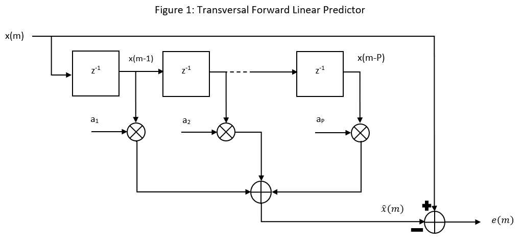
To obtain the LP coefficients, the mean square prediction error (eq.1.2) must be minimized.

$E(e^{2}(m)) = E[(x(m)-\hat{x}(m))^{2}] = r_{xx}(0) - 2\mathbf{r}_{xx}^{T}\mathbf{a} + \mathbf{a}^{T} \mathbf{R}_{xx}\mathbf{a}$ (eq. 1.2)

Here, $\mathbf{R}_{xx} = E(\mathbf{x}\mathbf{x}^{T})$ is the autocorrelation matrix of the signal vector $\mathbf{x}^{T}$ = [x(m-1) x(m-2) …x(m-P)] and $\mathbf{r}_{xx} = E(x(m)\mathbf{x})$ is the autocorrelation vector of x. By setting the gradient of eq. 1.2 equal to zero, the solution to the least mean square error problem is obtained. The solution to eq. 1.3 is given by eq. 1.4

$\frac{\partial }{\partial \mathbf{a}}E(e^{2}(m)) = -2\mathbf{r}_{xx}^{T}\mathbf{a}+2\mathbf{a}^{T}\mathbf{R}_{xx} = 0$ (1.3)

The solution to the above equation is given by:

$\mathbf{a} = \mathbf{R}_{xx}^{-1}\mathbf{r}_{xx}$ (1.4)

This solution can be expanded as:

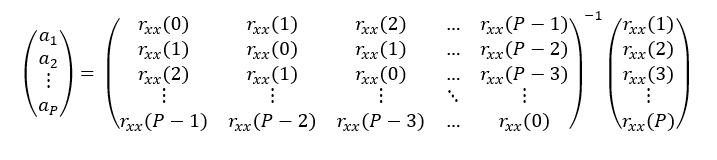
Solving the system above results in the solution to the Weiner-Hopf equation which yields the effective coefficients for the transversal forward linear prediction filter. For a more computationally efficient method of solving this equation (eq. 1.4), the Levinson-Durbin algorithm may be applied.

Complete Communications Engineering