In many cases, this can be done with an energy analysis. In a physical system, the total energy will be constant. Given a system state, it should be possible to calculate the total energy of the system. For a discrete time-step simulation, there will be a set of rules that transform the state at one time to the state at the next time. In many cases, these rules can be analyzed to calculate the change in energy from one time-step to the next. This can provide clues about whether the simulation will be stable or not.
An example will help to illustrate this analysis process. The example presented here is a simple harmonic oscillator. The oscillator is implemented in C using the following source code:
#include <stdio.h>
/* Spring constant */ #define SC 0.9
void main (void) { double x, v, a; /* position, velocity, acceleration */ double xn, vn; /* next position and velocity */ int i;
/* initial state */ x = 1.0; v = 0.0;
for (i = 0; i < 1000; i++) { a = -(x * SC); /* acceleration from spring force */ vn = v + a; /* next velocity */
/* two ways to calculate next position */ //xn = x + v; /* unstable */ xn = x + vn; /* stable */
/* update position and velocity */ x = xn; v = vn;
/* print position */ printf(“%f\n”, x); } } |
The oscillator is modeled as a mass on a spring, with the usual restoring force of -kx. The mass is assumed to be 1 (ignored). The code shows two different ways to calculate the next position of the mass. One uses the velocity from the current time-step (method A), the other uses the velocity from the next time-step (method B). When running the program, it is clear that method A is unstable, but method B appears to be stable. An energy analysis can help in understanding why this is so.
First, an expression is needed to calculate the system’s energy given its state. This system has two state variables that contribute to its energy: x and v. The potential energy (PE) is from x, and the kinetic energy (KE) is from v. The total energy is the sum. The following equation will be used to calculate the energy:
![]()
![]()
Next, the update rules need to be defined. These are the rules that calculate the next state given the current state. For this example, the following equations are used:

With this information, the energy of the next state can be calculated  . Subtracting the energy from the current state
  gives the change in energy
  .
.

The expressions (A2) and (B2) show how the energy of the system will change in the next time-step compared to the current time-step. Since k is a constant, these expressions have two variables, x and v. As the simulation progresses, the mass will follow some path through this 2D space and will gain or lose energy depending on the value of . Evaluating these expressions at x=0 and v=0 can give some insight into how the energy will change overall. The result is:
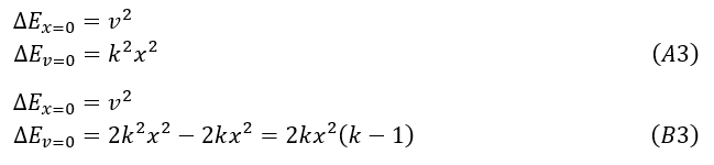
These results show that both systems gain energy when x=0. However, the change in energy differs when v=0. If method A is used, the energy always increases when v=0. Since it also increases when x=0, this is a clue that method A might be unstable. If method B is used, the energy can decrease when v=0. It will decrease as long as k < 1. This does not prove that method B is stable, but it is a clue that method B is more stable than method A.
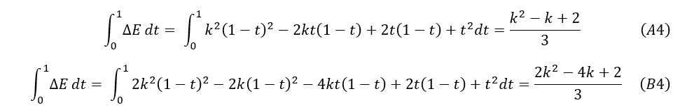
More evidence can be gained by integrating the change in energy expression across a path. This is a way to approximately calculate the total change in energy as the system moves from one state to another. Since a discrete simulation will not follow a continuous path this is only a heuristic but it does give more information about the difference in stability between method A and method B. The following path will be used for this example:

This is a straight line from (x = 1, v = 0) to (x = 0, v = 1). The actual simulation will not follow this path, but the integral does provide information about the change in energy at all points along the path. The integration results are as follows:
Plotting the final expressions (A4) and (B4) gives the following graph:
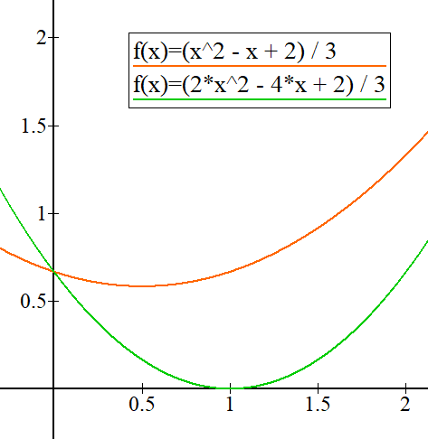
The graph for method A never gets close to zero, but the graph for method B reaches zero when k = 1. This is more evidence that as method A moves through its parameter space, it is constantly gaining energy which makes it unstable. As method B moves, it is also gaining energy but the gain is much less. Near k = 1 the energy gain is very close to zero. Again, this shows that method B is more stable than method A.