Time Delay Estimation

In signal processing, we often encounter problems that the time delay of a signal is required to perform certain operation. The signal model is usually modeled as below,

$y\left(t\right)=\alpha x\left(t-T_d\right)+n\left(t\right)$

The pure delay term, $T_d$ , can be used for many applications such as system diagnosis, radar ranging, direction of arrival, velocity measurement etc. More generally, we may model multipath channel as below,

$y\left(t\right)=\sum_{i\ =\ 1}^{M}{\alpha_ix\left(t-T_i\right)}+n\left(t\right)$

In this paper we only consider algorithms that can handle time delay being fractional. The problem can be formulated as below. The short duration signal shown in Figure 1 a) is the generating signal $x(t)$ , and Figure 1, b) is the delayed signal $y(t)$ .

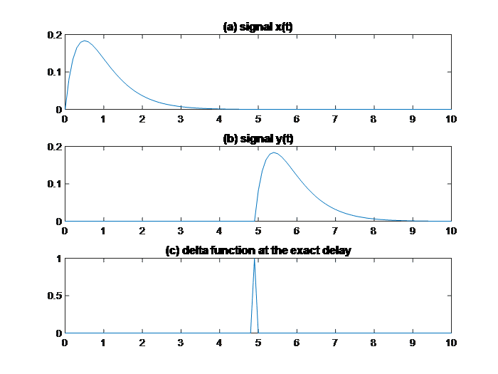
The signal $y(t)$ and $x(t)$ can be mathematically connected by an impulse function, as shown in Figure 1 c), through convolution,

$y\left(t\right)=\alpha\delta\left(t-T_d\right)\ast x\left(t\right)+n\left(t\right)$

In reality, $(t)$ may or may not be available. Our goal is to recover the impulse response function $\delta\left(t-T_d\right)$

.
We ignore the noise term $n(t)$ for simplicity. In frequency domain,

$Y\left(f\right) = X\left( f \right) e^{\left(j2\pi T_d\right)}$

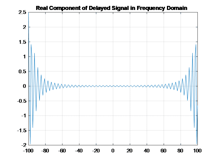
and if we take the real component only,

$Re\{Y\left(f\right)\}=Real\{A\left(f\right)\}cos\left(2\pi T_df+\phi\left(f\right)\right)$

Figure 2 shows the sinusoidal nature of the delayed signal in the frequency domain. Naturally one more layer of frequency transform will yield the period which is the delay we desire. However, due to the dramatic variation of frequency domain representation, we may apply logarithm operation before converting to the second layer frequency domain. The same practice is often used in cepstral analysis.

Complete Communications Engineering

Time Delay Estimation